Find where coverage drops

Steps

1. 01

   Load the reads

   Open the Workflow Builder at biochef.app. In File manager, upload run2-reads.fastq and phix174.fasta, and tick the reads for the Input node. New to the editor? The map reads tutorial shows each move with screenshots.

2. 02

   Map and sort

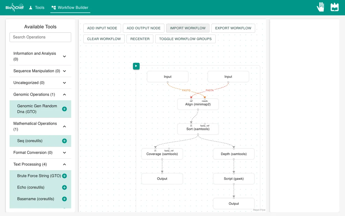
   Add Align (minimap2) with the reads in reads and a second Input with phix174.fasta in ref, switch on sam_output, then add Sort (samtools).

3. 03

   Get the overall coverage

   Select Sort and add Coverage (samtools) with an Output. It gives one summary line per sequence: reads, bases covered, percentage covered and mean depth.

4. 04

   Get the depth at every position

   Select Sort again and add Depth (samtools). Switch on all_positions so that positions with no reads are listed too, with depth 0. The output has one line per position: sequence name, position, depth.

5. 05

   List the low-coverage regions

   After Depth, add Script (gawk) and, in its required program field, paste:
   $3 < 10 { if (!s) s = $2; e = $2; next } s { print $1, s, e; s = 0 } END { if (s) print $1, s, e }
   For each run of positions with depth below 10, it prints where the run starts and ends. Add an Output and press ▶.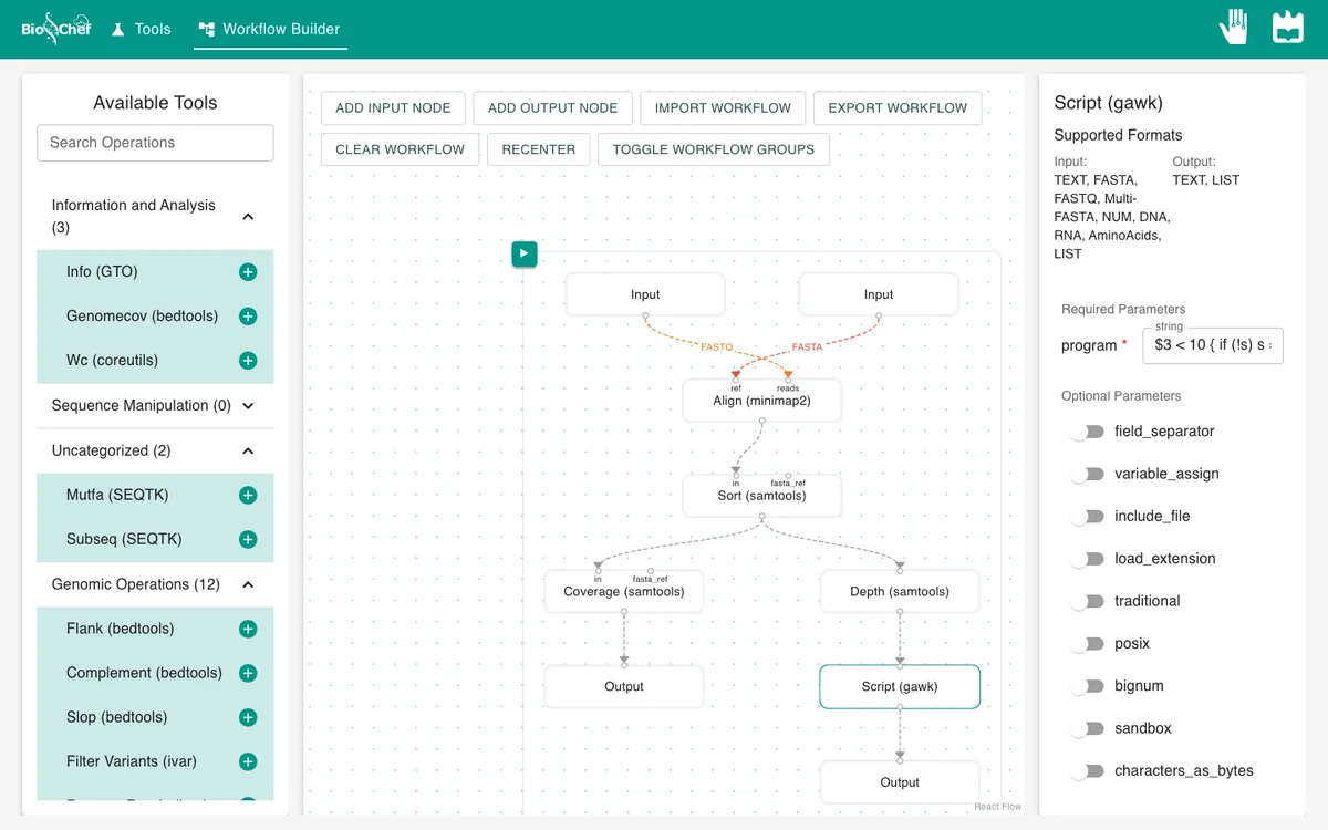

   

6. 06

   Read both results

   Click the two Outputs: the coverage summary, and the list of low-coverage regions.

   

#rname       startpos endpos numreads covbases coverage meandepth
NC_001422.1  1        5386   1000     5100     94.6899  27.8455

NC_001422.1 1 50
NC_001422.1 2301 2450
NC_001422.1 5301 5386